This is an old version of the class, kept for posterity. If you're seeing this, you probably want to check the URL and go to the latest version.

Ego Networks Activity

We read about the ego networks of Americans. In this exercise, you’ll create your own ego network and visualize it, using the skills that we’ve been working on in R.

First, you should create your network spreadsheets in Excel. Start by making a node attributes file with a row for each person that you have “discussed important matters with” over the last 6 months.

The columns of the spreadsheet should be: - name - gender - education (years of education) - race - age - is.kin (are they related to you?)

For is.kin, write TRUE if they are related to you and FALSE if they are not. Then, make a spreadsheet that’s an edgelist with a row for each connection in your network. For each edge, put the edge weight as 0 if they are strangers, 2 if they are especially close, or 1 if they are somewhere in between.

It should look something like this:

from	to	weight
Person 1	Person 2	1
Person 1	Person 3	2
Person 2	Person 3	0

…

Change the code below so that the path points to where you saved the edgelist and node attribute files.

edges <- read_excel('/home/jeremy/Teaching/can-s25.jeremydfoote.com/assignments/r_lab_examples/ego_edges.xlsx')
nodes <- read_excel('/home/jeremy/Teaching/can-s25.jeremydfoote.com/assignments/r_lab_examples/ego_atts.xlsx')

Code to load the file into R and make it into a network object.

G <- graph_from_data_frame(d=edges, vertices = nodes, directed = F) |> as_tbl_graph()

Code to filter out the edges that have a weight of 0.

G <- G |>
  activate(edges) |>
  filter(!is.na(weight)) |>
  filter(weight != 0)

This code will make a plot of the network. You’ll learn soon how to do this on your own.

G |>
  ggraph(layout = 'stress') +
  geom_edge_fan(aes(width = weight), alpha = .3) +
  geom_node_point(aes(color = is.kin), size = 3) +
  geom_node_text(aes(label = name), repel = TRUE, size = 4) +
  scale_color_viridis_d() +
  scale_edge_width(range = c(1, 3))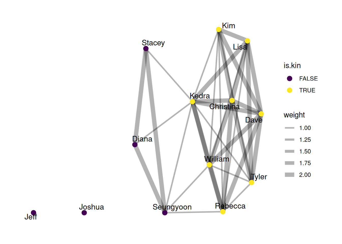

Exercises

Calculate the following for your network. Use Google to find the code to do this. I’ll give you the first one.

The number of nodes

G |>
  vcount()

[1] 13

The number of nodes who are kin (use the filter function)

[1] 8

The number of nodes who are non-kin

[1] 5

The density of the network

[1] 0.4615385

The standard deviation of age in your network.

As a hint, here’s how you would get the standard deviation of education

G |>
  activate(nodes) |>
  as_tibble() |>
  summarize(education_sd = sd(education))

# A tibble: 1 × 1
  education_sd
         <dbl>
1         5.46

# A tibble: 1 × 1
  age_sd
   <dbl>
1   15.5

What proportion of your network has the same race (the most common race)?

HINT: Here’s how you would get the proportion of the network that is kin.

G |>
  activate(nodes) |>
  as_tibble() |>
  summarize(kin_proportion = sum(is.kin == TRUE) / n())

# A tibble: 1 × 1
  kin_proportion
           <dbl>
1          0.615

# A tibble: 1 × 1
  same_race_proportion
                 <dbl>
1                0.923

What proportion of your network has the same gender (the most common gender)?

# A tibble: 13 × 6
   name      gender education race    age is.kin
   <chr>     <chr>      <dbl> <chr> <dbl> <lgl> 
 1 Kedra     F             16 W        38 TRUE  
 2 Rebecca   F              8 W        15 TRUE  
 3 Christina F             12 W        62 TRUE  
 4 Dave      M             15 W        66 TRUE  
 5 Lisa      F             16 W        36 TRUE  
 6 Kim       F             16 W        34 TRUE  
 7 Tyler     M             16 W        41 TRUE  
 8 Seungyoon F             22 A        46 FALSE 
 9 Jeff      M             22 W        48 FALSE 
10 Joshua    M             22 W        39 FALSE 
11 William   M              6 W        13 TRUE  
12 Stacey    F             22 W        55 FALSE 
13 Diana     F             22 W        40 FALSE

# A tibble: 1 × 1
  same_gender_proportion
                   <dbl>
1                  0.385